Linear Regression: Jupyter Notebook

pandas.DataFrame

Reading Data

Using read_csv() from pandas, read data into dataframe. If your data happens to be in a M$ Excel file, then there is also a read_excel() function.

import pandas as pd

dataset = pd.read_csv('./history_data.csv')

Relationship Between pandas.DataFrame and numpy.ndarray

See how a DataFrame holds values using numpy.ndarray.

dataset.values

array([['New York', 'New York', nan, ..., 0.0, nan, 'Clear'],
       ['New York', 'New York', nan, ..., 0.0, nan, 'Clear'],
       ['New York', 'New York', nan, ..., 0.0, 87.77, 'Clear'],
       ...,
       ['New York', 'New York', nan, ..., 23.3, 74.96, 'Clear'],
       ['New York', 'New York', nan, ..., 14.3, 70.33, 'Clear'],
       ['New York', 'New York', nan, ..., 0.0, 84.26, 'Clear']],
      dtype=object)

type(dataset.values)

numpy.ndarray

For convenience, pandas.DataFrame provides many attributes from the underlying numpy.ndarray.

Two dimensional array …

dataset.ndim

2

… extending such and such cell in each direction …

dataset.values.shape

(72, 16)

dataset.shape

(72, 16)

DataFrame.describe() is convenient for interactive use in a Jupyter notebook, just like many other methods.

dataset.describe()

	Resolved Address	Maximum Temperature	Minimum Temperature	Temperature	Wind Chill	Heat Index	Precipitation	Snow Depth	Wind Speed	Wind Gust	Cloud Cover	Relative Humidity
count	0.0	72.000000	72.000000	72.000000	0.0	22.000000	72.000000	0.0	72.000000	65.000000	72.000000	38.000000
mean	NaN	82.995833	70.688889	76.287500	NaN	91.327273	0.012222	NaN	12.690278	20.470769	3.369444	72.513421
std	NaN	5.946106	5.574023	5.313256	NaN	5.994536	0.070695	NaN	6.025980	8.302423	7.214825	12.665492
min	NaN	69.900000	53.300000	61.500000	NaN	82.400000	0.000000	NaN	2.200000	4.700000	0.000000	46.090000
25%	NaN	79.050000	68.900000	74.300000	NaN	87.050000	0.000000	NaN	9.100000	15.000000	0.000000	66.377500
50%	NaN	83.750000	71.950000	76.650000	NaN	89.750000	0.000000	NaN	12.800000	19.700000	0.000000	72.330000
75%	NaN	87.950000	74.325000	79.850000	NaN	95.950000	0.000000	NaN	15.425000	25.300000	2.825000	81.715000
max	NaN	92.900000	80.700000	85.800000	NaN	101.600000	0.470000	NaN	38.000000	50.600000	34.500000	96.970000

Extracting Input and Output Features from a pandas.DataFrame

Beware that algorithms expect a two dimensional array as the set of inputs. Using the column header (“Minimum Temperature”) to index the dataframe gives a list-like type. Wrong!!

inputfeatures = dataset['Minimum Temperature']

inputfeatures

0     53.3
1     58.7
2     60.2
3     66.8
4     68.3
      ...
67    70.1
68    72.2
69    72.1
70    75.5
71    78.2
Name: Minimum Temperature, Length: 72, dtype: float64

type(inputfeatures)

pandas.core.series.Series

Correction: index the dataframe with a list of column headers

inputfeatures = dataset[['Minimum Temperature']]

Sign of correctness: that one is made up more nicely by the notebook:

inputfeatures

	Minimum Temperature
0	53.3
1	58.7
2	60.2
3	66.8
4	68.3
...	...
67	70.1
68	72.2
69	72.1
70	75.5
71	78.2

72 rows × 1 columns

Likewise, the output features.

outputfeatures = dataset[['Maximum Temperature']]

Plotting with matplotlib

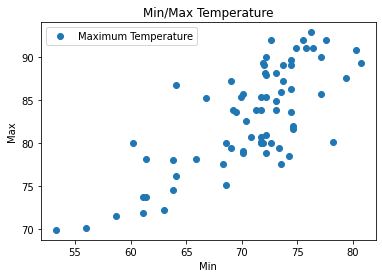
Fortunately (well, that was on purpose), our feature sets are one dimensional, so plotting the dataset im two dimensions makes sense. Multidimensional data analysis is not so straightforward - this is why they call it data science.

import matplotlib.pyplot as plt

pandas.DataFrame interacts nicely with matplotlib.

dataset.plot(x='Minimum Temperature', y='Maximum Temperature', style='o')
plt.title('Min/Max Temperature')
plt.xlabel('Min')
plt.ylabel('Max')
plt.show()

Data Splicing: Split into Training and Test Data

Before creating the model (from an algorithm and a dataset), we prepare the dataset * 80% for training * 20% for testing/verification

import sklearn
from sklearn.model_selection import train_test_split

input_train, input_test, output_train, output_test = \
     train_test_split(inputfeatures, outputfeatures, test_size=0.2, random_state=0)

Creating the Model: Algorithm + Training Data

from sklearn.linear_model import LinearRegression

Initially, the model is the algorithm

model = LinearRegression()

Next, we feed it the training data

model = model.fit(input_train, output_train)

Model is complete; see the parameters of the linear interpolation (would need theory to better understand):

model.coef_

array([[0.80189231]])

model.intercept_

array([25.95355086])

Verify the Model

We saved 20% of the dataset for verification. * Use the model to predict the output for the input test data. * Compare prediction to actual output test set

output_predicted = model.predict(input_test)

Here we (ab)use a pandas.DataFrame to nicely format actual output test data and predicted output side by side.

Note that input_test is a pd.DataFrame, but output_predicted is a numpy.ndarray.

Reason:model.predict() is happy with anything that supports indexing (thanks to duck typing - we gave it a Dataframe), but its output is always a numpy.ndarray

pd.DataFrame({'Actual': output_test.values.reshape((15,)),
              'Predicted': output_predicted.reshape((15,))})

	Actual	Predicted
0	80.0	83.609608
1	84.9	84.571879
2	91.1	86.736988
3	80.0	84.170933
4	78.2	78.798254
5	92.0	84.170933
6	78.2	75.189739
7	92.0	88.180394
8	85.4	83.449230
9	80.1	88.661530
10	92.9	87.057745
11	85.4	83.850176
12	87.2	81.284120
13	90.0	83.850176
14	83.6	81.685067

Comparing the actual and predicted values, we can see that they are “not far off”. Whatever this means - in a real data science world (this is only the surface), we would now have to use advanced statistical methods to actually measure the term “not far off”.

But this is left to data scientists. Our job is to create correct programs, and to keep those maintainable.