Goals of this Training#
Use Python to combine powerful libraries
Numerical: Pandas, NumPy
Scikit-Learn
Image Manipulation
Know what you are doing
Appreciate the beauty of the language
Jupyter Notebooks are also very cool
Exercise#
Load spectral image from a matlab file (.mat) into a 3-dimensional matrix. (See
scipy.io.loadmat)Use the K-Means algorithm to find clusters in the image. (See
sklearn.cluster.KMeans)Do something with that information. E.g. create a picture where the spectral pixels are converted to a RGB image of the same (x,y) dimension.
Links#
Basics
Documentation and Tutorials
Python
Numpy and all that
-
Numpy Arrays. Watch out for “boolean masking and advanced indexing” at around 50’.
-
Spyder vs. PyCharm. Spyder tries really hard to make global variables even more global, by retaining them in a context that it reuses between program invocations. The cited comparison is really comprehensive, but still nobody seems to have a problem with that misfeature.
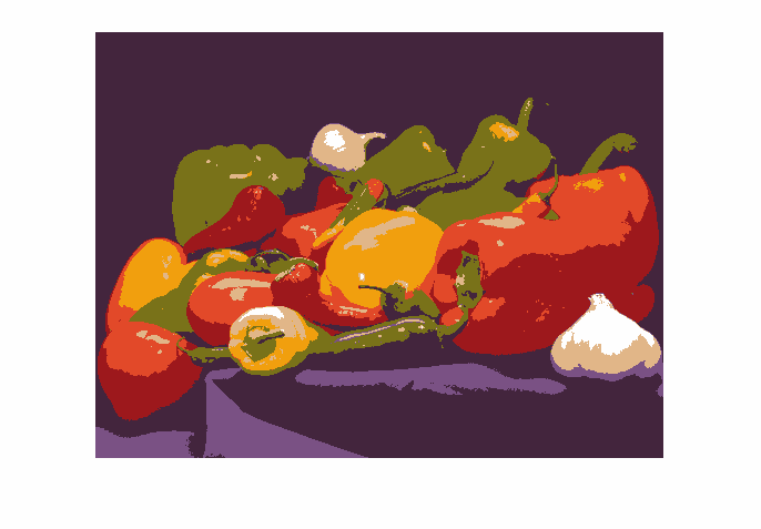
Walkthrough: Reduce Image to Eight Colors#
A related but more obvious problem is: given an RGB image, reduce colors to, say, eight.
Load PNG image into NumPy array
Make sense of it
Use K-Means to find eight clusters
Reduce colors by assigning center’s RGB to members
Convert NumPy array back into PNG
[1]:
IMGFILE = 'veggie.png'
Load Image from File: PIL#
Rant#
PIL was the original Python Imaging Library
For some reason a fork was created
Takes a while to learn to interpret Google search hits in this way
Welcome to Open Source
[2]:
import PIL.Image

img = PIL.Image.open(IMGFILE)
[3]:
img
[3]:
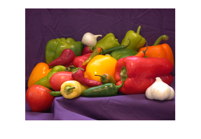
Image as NumPy Array#
This is easy: PIL is there to cooperate with numpy. The array shape, in this image’s case, is 477x686 for the x and y image dimensions, and 4 high for the (r,g,b,alpha) part.
[4]:
import numpy
imgarray = numpy.array(img)
[5]:
imgarray.ndim
[5]:
3
[6]:
imgarray.shape
[6]:
(477, 686, 4)
[7]:
imgarray.dtype
[7]:
dtype('uint8')
[8]:
imgarray
[8]:
array([[[255, 255, 255, 255],
        [255, 255, 255, 255],
        [255, 255, 255, 255],
        ...,
        [255, 255, 255, 255],
        [255, 255, 255, 255],
        [255, 255, 255, 255]],

       [[255, 255, 255, 255],
        [255, 255, 255, 255],
        [255, 255, 255, 255],
        ...,
        [255, 255, 255, 255],
        [255, 255, 255, 255],
        [255, 255, 255, 255]],

       [[255, 255, 255, 255],
        [255, 255, 255, 255],
        [255, 255, 255, 255],
        ...,
        [255, 255, 255, 255],
        [255, 255, 255, 255],
        [255, 255, 255, 255]],

       ...,

       [[255, 255, 255, 255],
        [255, 255, 255, 255],
        [255, 255, 255, 255],
        ...,
        [255, 255, 255, 255],
        [255, 255, 255, 255],
        [255, 255, 255, 255]],

       [[255, 255, 255, 255],
        [255, 255, 255, 255],
        [255, 255, 255, 255],
        ...,
        [255, 255, 255, 255],
        [255, 255, 255, 255],
        [255, 255, 255, 255]],

       [[255, 255, 255, 255],
        [255, 255, 255, 255],
        [255, 255, 255, 255],
        ...,
        [255, 255, 255, 255],
        [255, 255, 255, 255],
        [255, 255, 255, 255]]], dtype=uint8)
[9]:
imgarray[200,300] # arbitrary pixel somewhere in the middle
[9]:
array([172, 104, 25, 255], dtype=uint8)
Preparation before Clustering#
Cut off Alpha plane
Clustering input: only “3d” RGB values
[10]:
rgb = imgarray[:,:,0:3]
alpha = imgarray[:,:,3]
[11]:
rgb.shape
[11]:
(477, 686, 3)
[12]:
# remember for later
nrows, ncols, _ = rgb.shape
[13]:
alpha.shape
[13]:
(477, 686)
While we have compatible x,y sizes, we are missing one dimension in the alpha matrix. We need this to stack alpha on top of the reduced image once we have it.
[14]:
alpha = alpha.reshape(alpha.shape + (1,))
This could have been done easier by slicing a range of size 1 instead …
[15]:
alpha = imgarray[:,:,3:]
[16]:
alpha.shape
[16]:
(477, 686, 1)
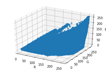
Excursion: matplotlib#
Completely irrelevant: see where the points are in the RGB colorspace. Could spend more time on it though; for example, the points could be colored.
[17]:
%matplotlib inline

from mpl_toolkits.mplot3d import Axes3D
import matplotlib.pyplot as plt

fig = plt.figure()
ax = fig.add_subplot(111, projection='3d')
ax.set_xlabel('R')
ax.set_ylabel('G')
ax.set_zlabel('B')
[17]:
Text(0.5, 0, 'B')
[18]:
rs = []
gs = []
bs = []
for x, y in numpy.ndindex(nrows,ncols):
    r,g,b = rgb[x,y]
    rs.append(r)
    gs.append(g)
    bs.append(b)
[19]:
ax.scatter(rs,gs,bs)
fig
[19]:
Now Comes the Clustering#
Huge data science toolbox
K-Means: “Given a set of data points, find N clusters and their centers”
We have a two-dimensional array of (r,g,b) values. KMeans is not interested in (x,y), so linearize the input. Note that reshaping an array is a zero-copy operation - it only gives a different view onto the same memory.
[20]:
rgb_linear = rgb.reshape(nrows*ncols, 3)
Let KMeans find eight clusters …#
[21]:
from sklearn.cluster import KMeans

km = KMeans(n_clusters=8)
km.fit(rgb_linear)
[21]:
KMeans(algorithm='auto', copy_x=True, init='k-means++', max_iter=300,
       n_clusters=8, n_init=10, n_jobs=None, precompute_distances='auto',
       random_state=None, tol=0.0001, verbose=0)
Use the result: output-properties#
labels: cluster membership for each point in the input sequence
cluster_centers: eight RGB values
[22]:
km.labels_
[22]:
array([1, 1, 1, ..., 1, 1, 1], dtype=int32)
[23]:
len(km.labels_)
[23]:
327222
[24]:
nrows*ncols
[24]:
327222
[25]:
km.cluster_centers_
[25]:
array([[ 67.20529747,  37.50360681,  61.3796182 ],
       [254.94408609, 254.75471018, 254.53133237],
       [226.64913628,  73.76939951,  41.92569235],
       [121.71464963, 114.47333306,  25.60640492],
       [122.8888303 ,  81.92275244, 132.84313209],
       [157.30685398,  24.43988931,  28.03959132],
       [225.55934051, 182.98255893, 136.3232048 ],
       [241.37322907, 159.54158234,  14.51775529]])
Clusters be their Centers#
Assign each point the RGB values of the center it is attached to
[26]:
for idx, label in enumerate(km.labels_):
    rgb_linear[idx] = km.cluster_centers_[label]
Post Processing: Restore Alpha, Back into RGBA#
Note: while we have manipulated the RGB cube via rgb_linear (a two-dimensional view of it), we use the original three-dimensional rgb array.
[27]:
imgarray = numpy.concatenate((rgb, alpha), axis=2)
[28]:
reduced_img = PIL.Image.fromarray(imgarray, 'RGBA')
[29]:
reduced_img
[29]: